Temporal Policy:
History Initialized Action Generation for Robotic Learning from Demonstration

Dylan Miller

Supervisor: Dr. Martin Jagersand

1. Introduction & Motivation

Learning from Demonstration (LfD)

The Goal: Teach robots complex behaviors directly from expert demonstrations.

LfD Benefits

• No Reward Engineering: Challenging to specify reward for real world manipulation tasks.
• Sample Efficiency: Learns complex tasks from a relatively small dataset of expert trajectories.
• Bypasses Analytical Modeling: Directly maps observations to actions, avoiding the need to build rigorous, mathematical models of contact dynamics and friction.

Collection Modalities

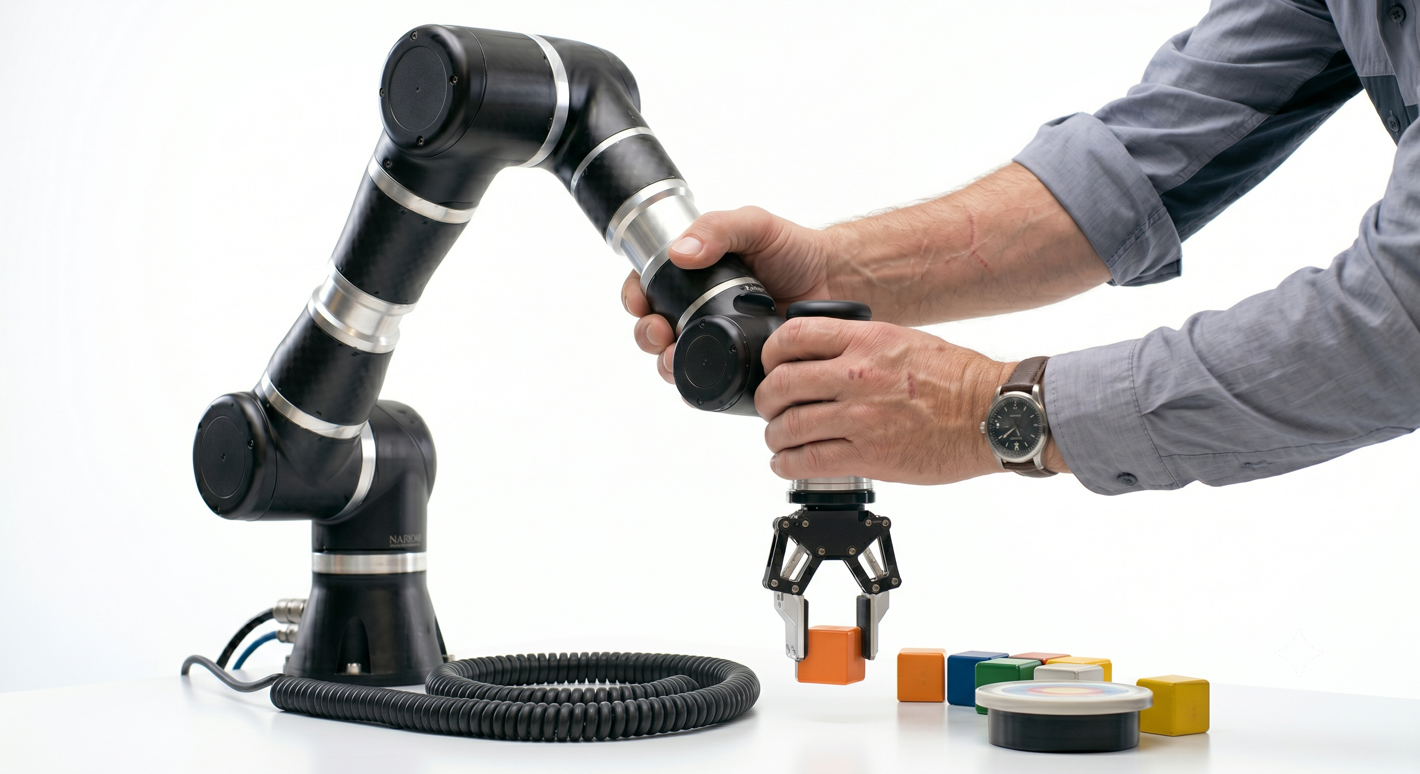
• Kinesthetic teaching

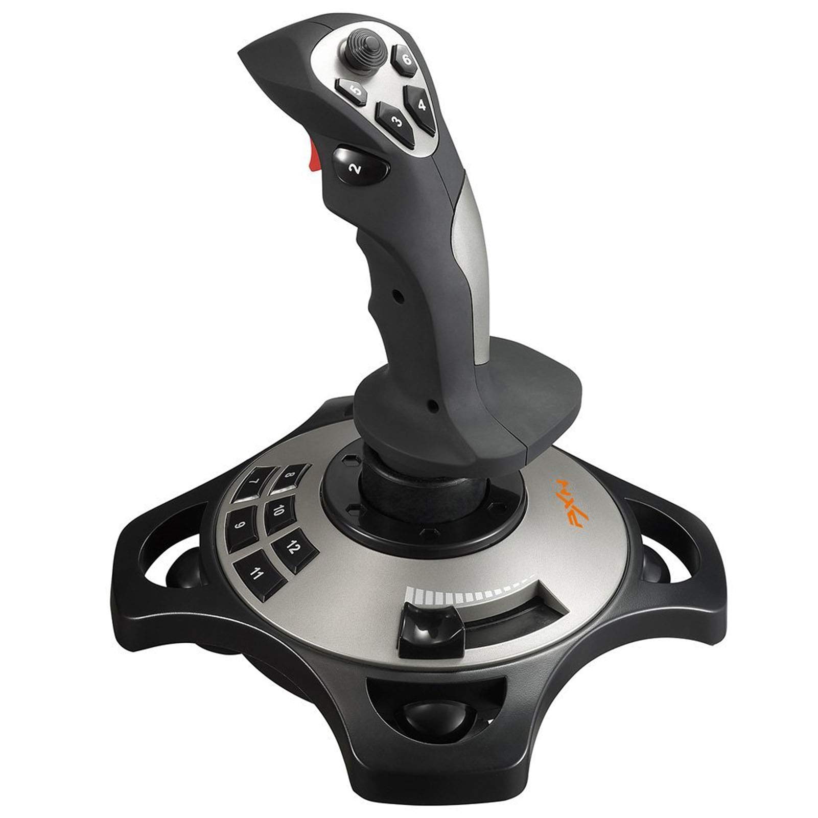
• Joystick

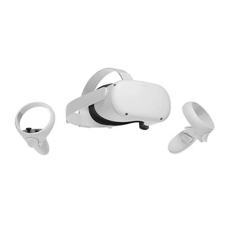
• VR

• Leader-Follower

Capturing the Demonstration Distribution

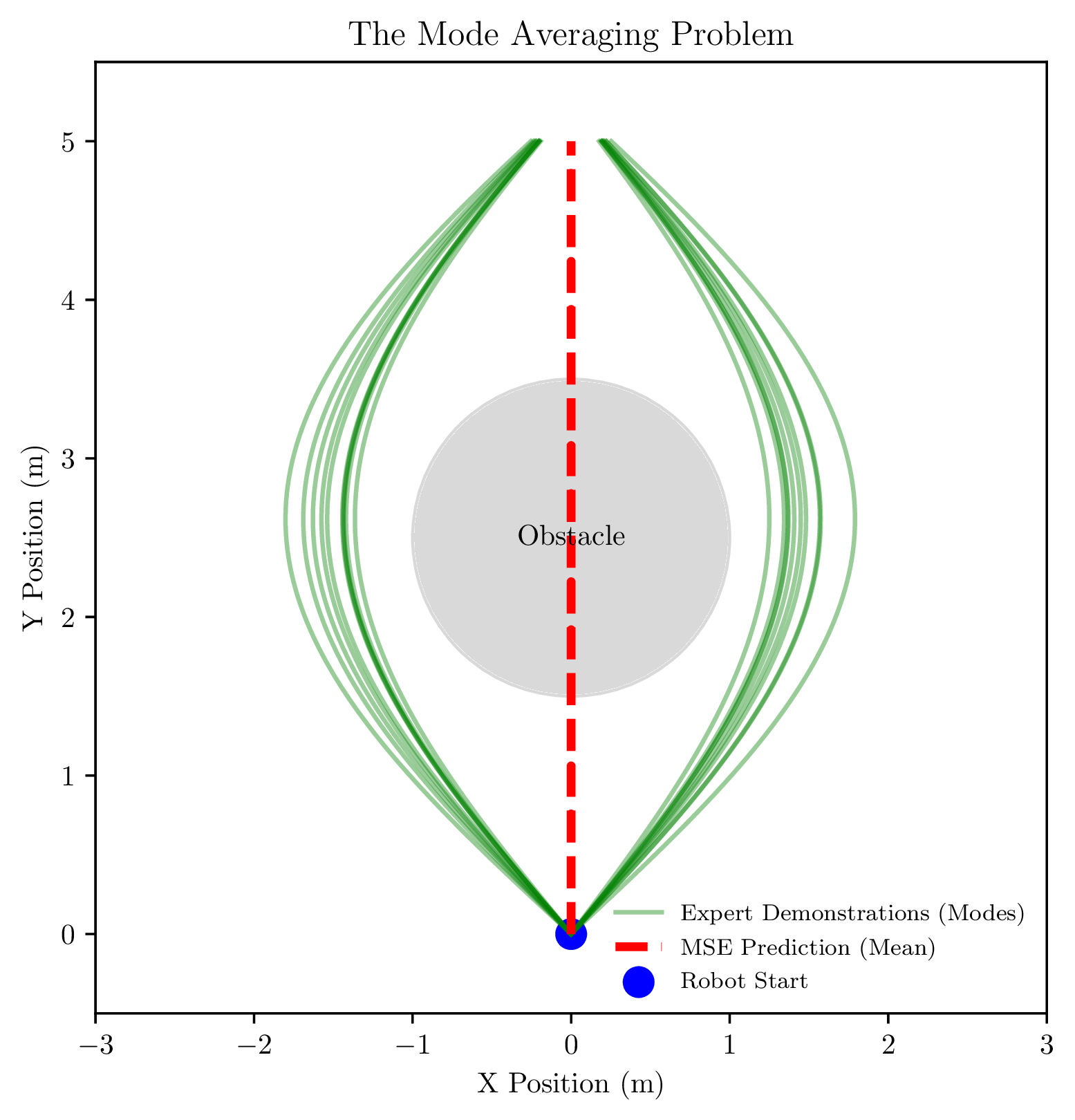
• Classical Behavior Cloning (suffers from mode-averaging).

• Generative Models: Capture rich, multimodal action distributions.

Diffusion Policy

One of the most successful generative models for robotic LfD

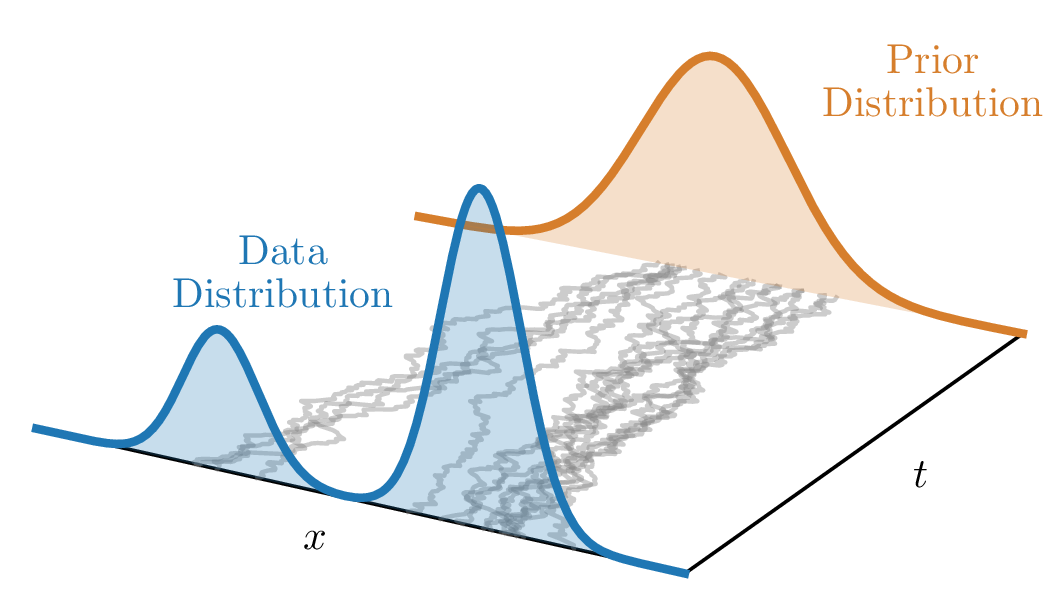
• Diffusion Model - Learns transformation from Standard Gaussian to data distribution
• Captures multimodal distributions
• Stable to train

(Chi et al. 2023)

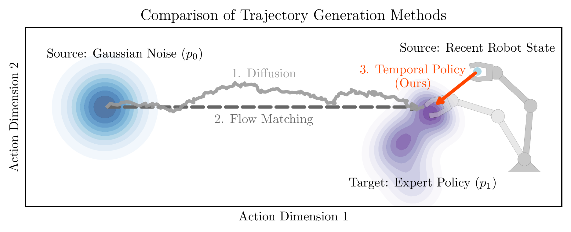
The Bottleneck: Noise-Initialized Models

• Uninformative Prior: Initialized from Standard Gaussian.
• Results in long, high-curvature transport paths.

• Impact:
  • Complex mapping
  • High inference latency
  • Poor interpretability

Towards Informative Priors

The field has recognized the bottleneck of pure noise initialization.

• Image domain example:
  • (Albergo et al. 2024) demonstrated informative starting states (e.g., mapping directly from a downsampled image to a upsampled image).
  • Result: Massive reductions in transport cost. Improved image generation.

Robotics Attempts

• VITA (Gao et al. 2026)
  • Transports image to action
  • Drawback: Numerical simulation during training, lacks physical interpretability.
• Streaming Flow Policy (Jiang et al. 2025)
  • Transports previous state to next state
  • Drawback: Only maps a single step instead of sequence of actions. Artificial mixing of behaviour.

Proposed Solution: Temporal Policy

Instead of mapping from noise to data, we map the past to the future.

• Core Insight: Initialize the generative process directly from the robot’s recent state history.
• The Framework: Formulated using Stochastic Interpolants.

Key Properties of Temporal Policy

• Short Transport Distance: Initializes directly at the recent state history, bypassing the large geometric gap of global noise.
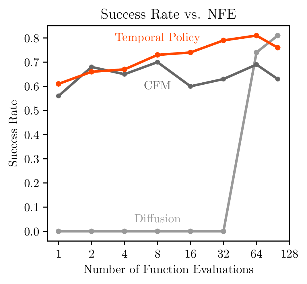
• Highly Linear Path: Straighter generative paths require fewer network evaluations (NFE).
• Flexible Inference: Supports both fast deterministic (ODE) sampling and robust stochastic (SDE) sampling.
• Stable Training: Vector fields are learned via direct regression, avoiding the instability of backpropagating through solvers.
• Interpretability: Unlike abstract noise spaces, the learned vectors represent grounded physical displacements.

2. Background & Theory

Stochastic Differential Equation (SDE)

\mathrm{d}\mathbf{x}_t = \underbrace{\mathbf{f}(\mathbf{x}_t, t)\mathrm{d}t}_{\text{Drift}} + \underbrace{g(t)\mathrm{d}\mathbf{w}_t}_{\text{Diffusion}}

• Drift: The deterministic vector field.
• Diffusion: Continuous noise injection enabling multimodal representation
• \mathbf{w}_t represents a standard Wiener process (Brownian motion), driven by continuous stochastic increments.

Continuous Diffusion Models

Diffusion models learn to reverse a noise injection process.

1. Forward Process: Systematically degrades data into an simple prior over time t \in [0, T] (where T \to \infty): \mathrm{d}\mathbf{x} = \mathbf{f}(\mathbf{x}, t)\mathrm{d}t + g(t)\mathrm{d}\mathbf{w}

2. Reverse Process: This process can be reversed (Anderson 1982): \mathrm{d}\mathbf{x} = [\mathbf{f}(\mathbf{x}, t) - g(t)^2 \nabla_{\mathbf{x}} \log p_t(\mathbf{x})]\mathrm{d}t + g(t)\mathrm{d}\bar{\mathbf{w}}

• Score Matching: We train a network to estimate the score \nabla_{\mathbf{x}} \log p_t(\mathbf{x}).

(Song et al. 2021)

Conditional Flow Matching (CFM)

CFM reframes generation as learning a deterministic vector field (ODE).

• The Linear Interpolant: Straight line connecting noise \mathbf{x}_0 to target data \mathbf{x}_1 \mathbf{x}_t = (1-t)\mathbf{x}_0 + t\mathbf{x}_1; \quad t \in [0,1]

• The Target Velocity: Constant straight line \mathbf{u}_t(\mathbf{x}|\mathbf{x}_0, \mathbf{x}_1) = \mathbf{x}_1 - \mathbf{x}_0

• The Objective: Train a network v_\theta to predict this straight-line velocity via MSE regression.

• Inference: Follow the predicted velocity field (Euler). \mathbf{x}_{t+\Delta t} = \mathbf{x}_t + v_\theta(\mathbf{x}_t, t) \Delta t

(Lipman et al. 2023)

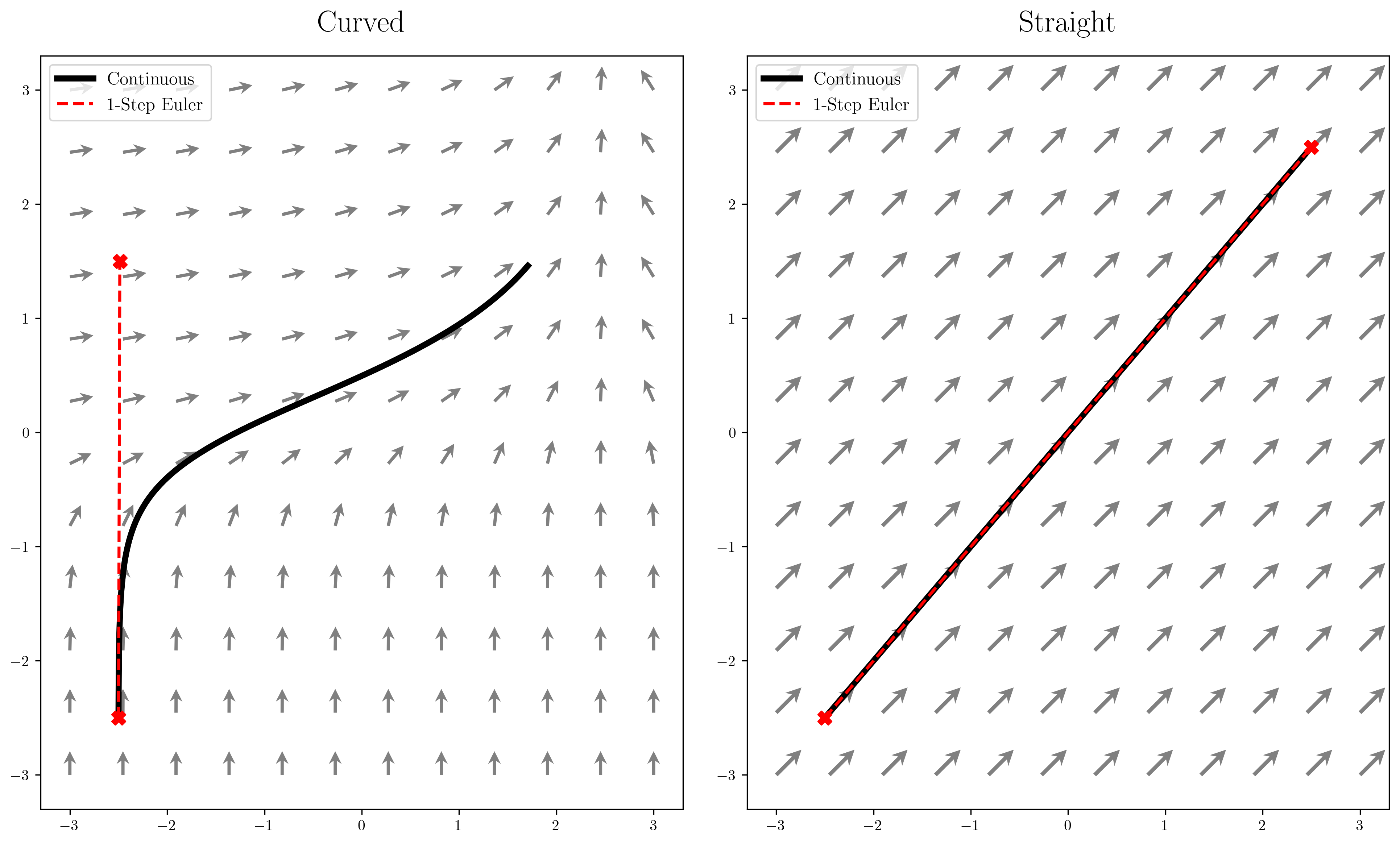
Vector Field

The Geometry of Couplings

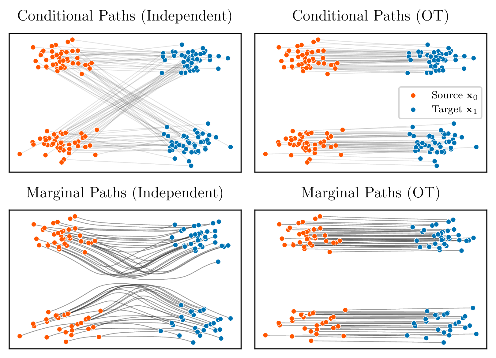
Coupling describes the joint distribution (x_0, x_1) \sim q(p_0, p_1)

1. Independent Coupling:

• Randomly pairs source x_0 with data x_1.

2. Optimal Transport (OT) Coupling:

• Minimizes path crossing by sorting source-to-data pairs.

3. Methodology: Temporal Policy

State & Action Representation

State and actions share the same representation

• e.g. Joint positions, Cartesian pose

Action Chunking Strategy

• Instead of predicting a single step a_t, we predict a horizon H of future actions.
  • Temporal Smoothness: Generates a cohesive trajectory.
  • Computational Efficiency: Amortizes the cost of network forward passes.

The Temporal Coupling Formulation

We exploit the temporal structure of expert demonstrations.

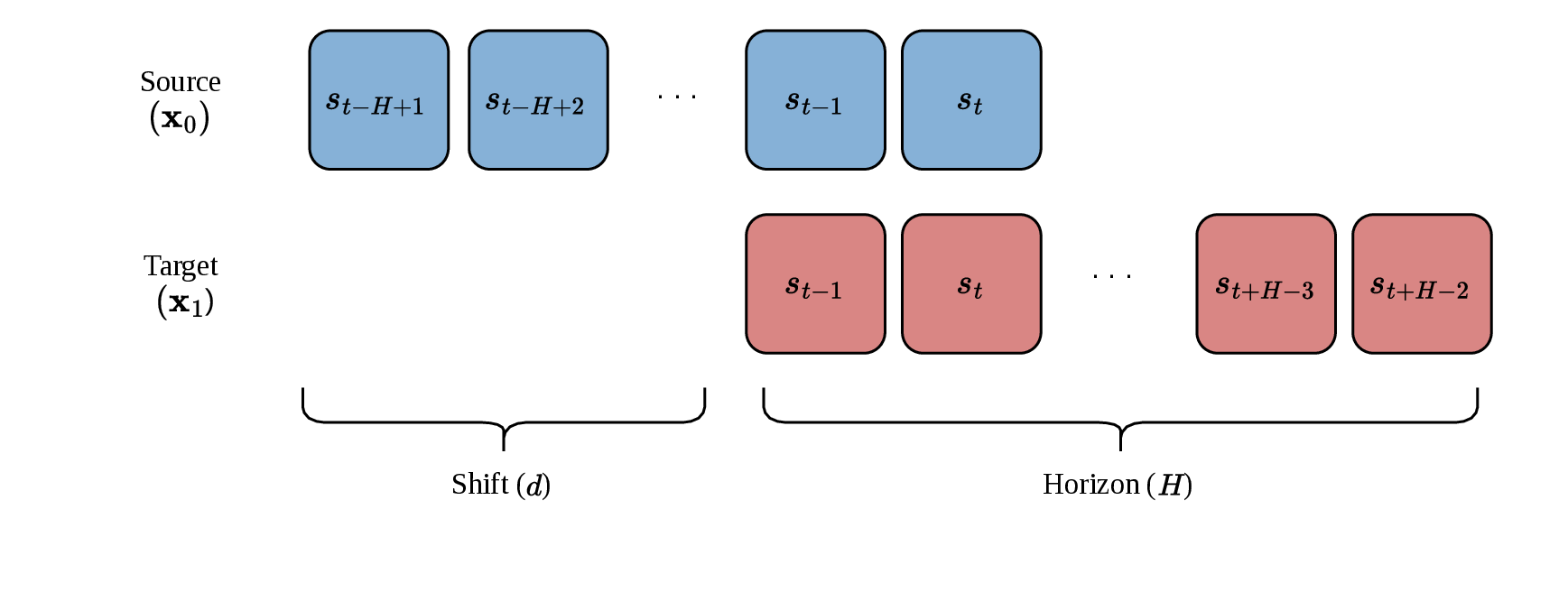
• Source (\mathbf{x}_0): Recent state history (s_{t-H+1:t}).
• Target (\mathbf{x}_1): Future action chunk (s_{t-H+1+d:t+d}).
• Overlap (d < H) reduces trajectory discontinuities.

The Stochastic Interpolant

We construct an interpolant that mixes the source, target, and a non-stationary Wiener process:

\mathbf{x}_\lambda = (1-\lambda)\mathbf{x}_0 + \lambda\mathbf{x}_1 + \epsilon(1-\lambda)\mathbf{w}_\lambda

Boundary Conditions:

• Start (\lambda=0): Exactly at history \mathbf{x}_0.
• End (\lambda=1): Exactly at target action \mathbf{x}_1.

(Chen et al. 2024)

Regression Target

\mathrm{d}\mathbf{x}_\lambda = \underbrace{\left[ (\mathbf{x}_1 - \mathbf{x}_0) - \epsilon \mathbf{w}_\lambda \right]}_{\text{Drift}} \mathrm{d}\lambda + \epsilon (1 - \lambda) \mathrm{d}\mathbf{w}_\lambda.

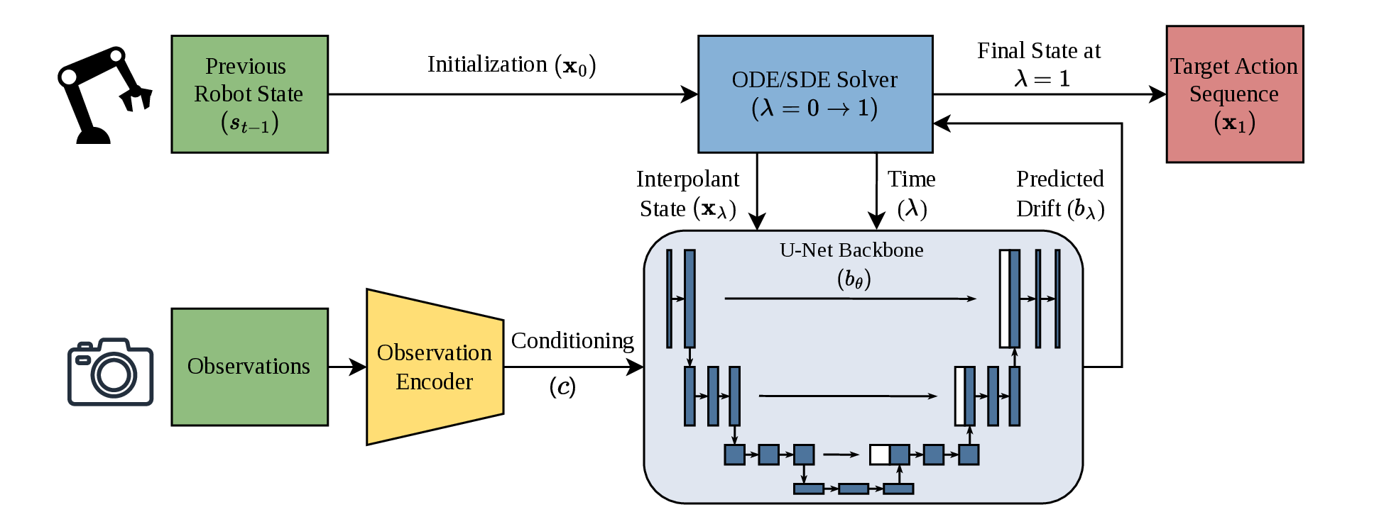
We train a neural network b_\theta to match the drift of the interpolant.

\mathbf{w}_\lambda \stackrel{d}{=} \sqrt{\lambda}\mathbf{z}; \quad \mathbf{z} \sim \mathcal{N}(\mathbf{0}, \mathbf{I})

\mathcal{L}(\theta) = \mathbb{E}_{\lambda, (\mathbf{x}_0, \mathbf{x}_1), \mathbf{z}} \left[ \left\| b_\theta(\mathbf{x}_\lambda, \mathbf{x}_0, \lambda) - \left( \mathbf{x}_1 - \mathbf{x}_0 - \epsilon \sqrt{\lambda}\mathbf{z} \right) \right\|^2 \right]

Network Architecture

• Observation Encoder: ResNet-18 (or similar) with Spatial Softmax.
• Sequence Modeling: 1D Convolutional U-Net.
• Conditioning: Sinusoidal embeddings from interpolation step \lambda + conditioning vector injected via FiLM layers.

SDE Inference: Euler-Maruyama

1. The Continuous SDE: \mathrm{d}\mathbf{x}_\lambda = b_{\theta}(\mathbf{x}_{\lambda}, \mathbf{x}_0, \lambda) \mathrm{d}\lambda + \epsilon (1 - \lambda) \mathrm{d}\mathbf{w}_\lambda.

2. The Discrete Update Step: \mathbf{x}_{\lambda+ \Delta \lambda} = \mathbf{x}_\lambda + \underbrace{b_{\theta}(\mathbf{x}_i, \mathbf{x}_0, \lambda_i)\Delta\lambda}_{\text{Deterministic Step}} + \underbrace{\epsilon (1 - \lambda)\sqrt{\Delta\lambda}\mathbf{z}_\lambda}_{\text{Noise Injection}}

• \Delta\lambda: The discretization step size.
• \mathbf{z}_\lambda \sim \mathcal{N}(\mathbf{0}, \mathbf{I})

Changing the Noise Schedule

We can change the noise schedule at inference time without retraining the network. \mathrm{d}\mathbf{x} = \underbrace{\left[ b_{\theta} + \frac{g_\lambda^2 - \gamma_\lambda^2}{2} \nabla_{\mathbf{x}} \log p_\lambda(\mathbf{x}|\mathbf{x}_0) \right]}_{\text{corrected drift }\tilde{b}} \mathrm{d}\lambda + g_{\lambda} \mathrm{d}\mathbf{w}

• g_{\lambda} - New noise schedule
• \gamma_{\lambda} - Training noise schedule

Flexible Inference: ODE vs SDE

Allows for two sampling modes:

1. Deterministic ODE: Requires fewer function evaluations. Yields a single, deterministic trajectory.
2. Stochastic SDE: Injects noise during sampling. Slower, but can generate diverse samples.

Overall Pipeline

4. Experiments

Simulation Benchmarks (Robomimic)

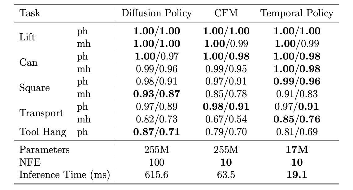
Evaluated across 5 tasks of varying complexity (Lift, Can, Square, Transport, Tool Hang).

Quantitative Success Rates

Temporal Policy matches state of the art success rates

Max/Average Success Rate

NVIDIA RTX 4080

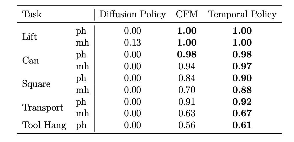
Inference Steps on Success Rate

Single integration step performance

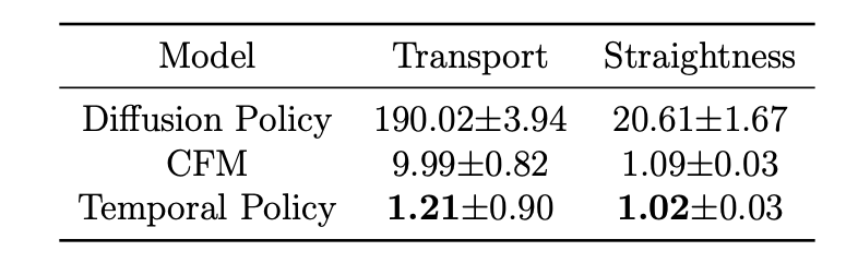
Visualizing Transport Path

Geometric Efficiency

• A Straightness ratio of 1.0 indicates a perfectly straight line.

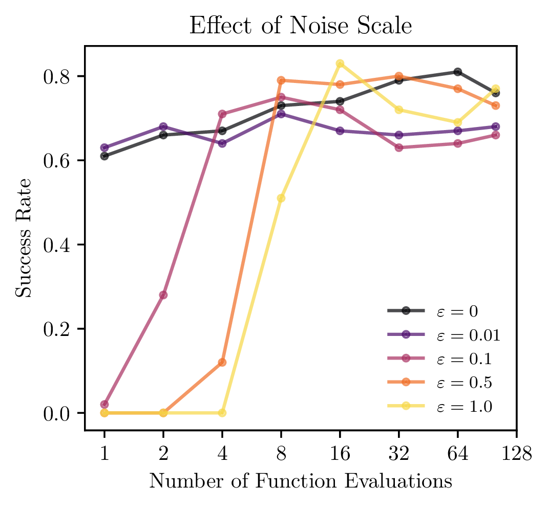
Ablation: Inference Noise Scale

• Rightward shift as \epsilon increases
• SDE does not show superior performance given computational trade off

Ablation: Training Noise Scale

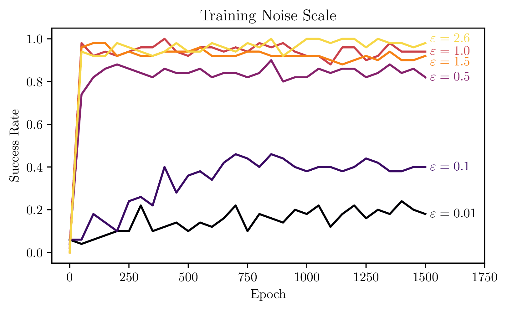
Recall: \mathbf{x}_\lambda = (1-\lambda)\mathbf{x}_0 + \lambda\mathbf{x}_1 + \epsilon(1-\lambda)\mathbf{w}_\lambda

• \epsilon \leq 0.1: Fails to learn a robust velocity field.
• \epsilon = 1.0: The empirical sweet spot. Induces enough noise to learn a corrective vector field without washing out the underlying trajectory signal.
• \epsilon > 2.0: Network wastes capacity on pure denoising.

Hardware Setup

• Leader Robot: 4-DoF Barrett WAM with custom 3-DoF wrist
• Follower Robot: 7-DoF Barrett WAM
• Perception: 2 RGB cameras (Wrist and 3rd-person).
• Expert Data: 150 demonstrations.

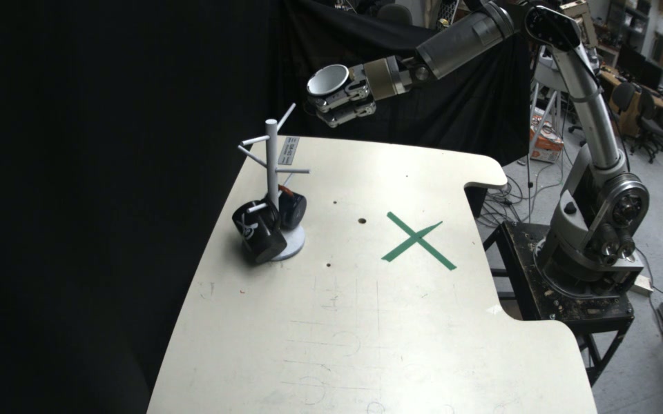
Hardware Validation: Mug-Hanging

• Success Rate:
  • 95% pick phase (19/20).
  • 50% overall (10/20)
• Latency: 19.62 ms
  • Well below 30 FPS camera rate.

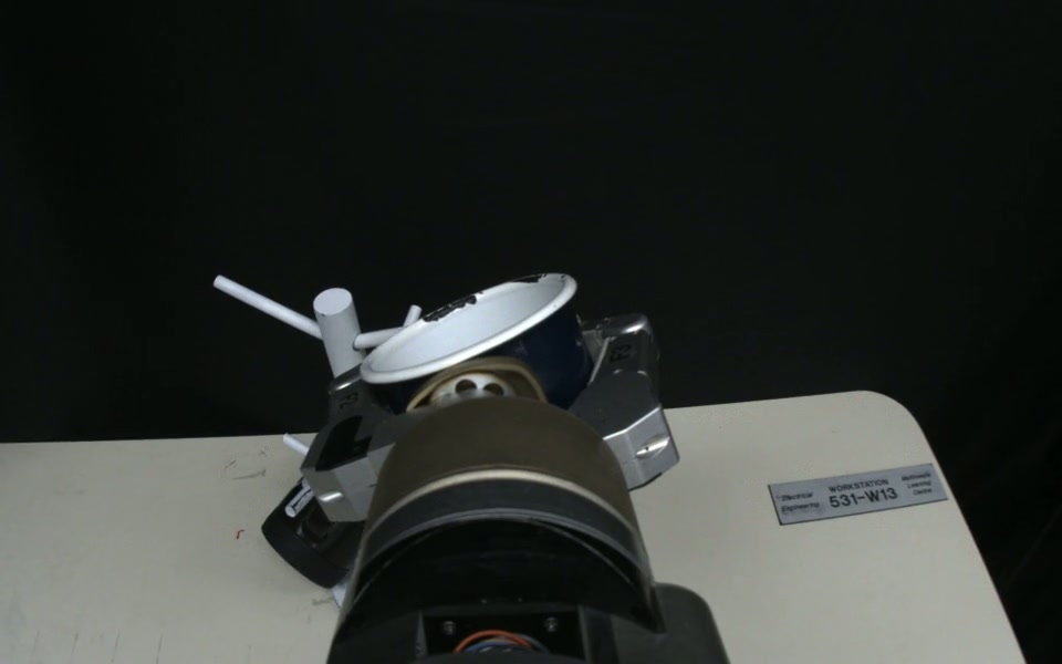
Analyzing Hardware Failures

• Visual Occlusion: . During the fine alignment phase, the grasped mug completely obstructed the wrist camera.

Key Properties of Temporal Policy

• Short Transport Distance: Initializes directly at the recent state history, bypassing the large geometric gap of global noise.
• Highly Linear Path: Straighter generative paths require fewer network evaluations (NFE).
• Flexible Inference: Supports both fast deterministic (ODE) sampling and robust stochastic (SDE) sampling.
• Stable Training: Vector fields are learned via direct regression, avoiding the instability of backpropagating through solvers.
• Interpretability: Unlike abstract noise spaces, the learned vectors represent grounded physical displacements.

Impact & Limitations

Impact:

• Shifts generative LfD from abstract denoising to a physically grounded transport process.
• Reduce the computational bottleneck that limits real-time control.

Limitations:

• Bound by expert data quality.
• Sensitivities to state initialization (perception noise, latency propagates directly).

Future Directions

• Additional Modalities: Integrating force, depth, and language conditioning.
• Velocity Projection: Projecting the initial state forward to further reduce transport cost.
• Exploiting physically grounded velocity field: Kinematic limits, obstacle avoidance.

Questions

References

Albergo, Michael Samuel, Mark Goldstein, Nicholas Matthew Boffi, Rajesh Ranganath, and Eric Vanden-Eijnden. 2024. “Stochastic Interpolants with Data-Dependent Couplings.” In Proceedings of the 41st International Conference on Machine Learning, 921–37. PMLR. https://proceedings.mlr.press/v235/albergo24a.html.

Anderson, Brian D. O. 1982. “Reverse-Time Diffusion Equation Models.” Stochastic Processes and Their Applications 12 (3): 313–26. https://doi.org/10.1016/0304-4149(82)90051-5.

Chen, Yifan, Mark Goldstein, Mengjian Hua, Michael Samuel Albergo, Nicholas Matthew Boffi, and Eric Vanden-Eijnden. 2024. “Probabilistic Forecasting with Stochastic Interpolants and Föllmer Processes.” In Proceedings of the 41st International Conference on Machine Learning, 6728–56. PMLR. https://proceedings.mlr.press/v235/chen24n.html.

Chi, Cheng, Siyuan Feng, Yilun Du, Zhenjia Xu, Eric Cousineau, Benjamin Burchfiel, and Shuran Song. 2023. “Visuomotor Policy Learning via Action Diffusion.” The International Journal of Robotics Research. https://arxiv.org/pdf/2303.04137.

Gao, Dechen, Boqi Zhao, Andrew Lee, Ian Chuang, Hanchu Zhou, Hang Wang, Zhe Zhao, Junshan Zhang, and Iman Soltani. 2026. “VITA: Vision-to-Action Flow Matching Policy.” arXiv. https://doi.org/10.48550/arXiv.2507.13231.

Jiang, Sunshine, Xiaolin Fang, Nicholas Roy, Tomás Lozano-Pérez, Leslie Pack Kaelbling, and Siddharth Ancha. 2025. “Streaming Flow Policy: Simplifying Diffusion/Flow-Matching Policies by Treating Action Trajectories as Flow Trajectories.” In Proceedings of The 9th Conference on Robot Learning, 238–57. PMLR. https://proceedings.mlr.press/v305/jiang25a.html.

Lipman, Yaron, Ricky T. Q. Chen, Heli Ben-Hamu, Maximilian Nickel, and Matt Le. 2023. “Flow Matching for Generative Modeling.” arXiv. http://arxiv.org/abs/2210.02747.

Song, Yang, Jascha Sohl-Dickstein, Diederik P. Kingma, Abhishek Kumar, Stefano Ermon, and Ben Poole. 2021. “Score-Based Generative Modeling Through Stochastic Differential Equations.” arXiv. http://arxiv.org/abs/2011.13456.

Extra Slides

Multimodal

The Probability Flow ODE

\mathrm{d}\mathbf{x}_t = \left[ \mathbf{f}(\mathbf{x}_t, t) - \frac{1}{2}g(t)^2 \nabla_{\mathbf{x}} \log p_t(\mathbf{x}_t) \right] \mathrm{d}t

Fokker-Planck Equation

\frac{\partial p_t(x)}{\partial t} = -\nabla_x \cdot (f(x,t) p_t(x)) + \frac{1}{2} g(t)^2 \Delta p_t(x)